Problem Description
A robot is located at the top-left corner of a m x n grid (marked 'Start' in the diagram below).
The robot can only move either down or right at any point in time. The robot is trying to reach the bottom-right corner of the grid (marked 'Finish' in the diagram below).
How many possible unique paths are there?
Example 1:
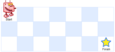
Input: m = 3, n = 7
Output: 28
Example 2:
Input: m = 3, n = 2
Output: 3
Explanation:
From the top-left corner, there are a total of 3 ways to reach the bottom-right corner:
1. Right -> Down -> Down
2. Down -> Down -> Right
3. Down -> Right -> Down
Example 3:
Input: m = 7, n = 3
Output: 28
Example 4:
Input: m = 3, n = 3
Output: 6
Constraints:
1 <= m, n <= 100- It's guaranteed that the answer will be less than or equal to
2 * 109.
The description was taken from https://leetcode.com/problems/unique-paths/.
Problem Solution
#O(M*N) Time, O(M*N) Spaceclass Solution: def uniquePaths(self, m: int, n: int) -> int: for col in range(1,m): for row in range(1,n): dp[col][row] = dp[col-1][row] + dp[col][row-1] return dp[m-1][n-1]Problem Explanation
Like Decode Ways, Climbing Stairs, House Robber, Paint the Fence, this problem falls in the Dynamic Programming category of finding a running combination. To solve these problems, we will arrive at point B and look back at each potential point A that we got here from, and add the combinations from our point A's to point B.
Let's think about just how the robot would get to the final cell in general.
If we only had one row, then the robot would just go to the right. If we only had one column, then the robot would just go down. That tells us that for each cell that the robot has traveled to, the robot must have gotten there from the cell above it or to the left of it.
To calculate this, we can perform tabulation in the form of bottom-up Dynamic Programming.
We will traverse the grid, and each time we arrive at a new cell, we will track the unique paths to get to that cell by incrementing the cell by the paths from the cell directly above it and the cell directly to the left of it.
Let's start by creating the grid.
This code above translates to "dp is an array of ones in the length of n, and we'll have m rows of that array."
dp = [[1]*n for rows in range(0,m)]
Next, we will traverse the columns and rows from index one because our base case would be one path if we received an m or n with the value of zero.
for col in range(1,m): for row in range(1,n):
For each cell index, we will increment its unique paths element by the amount in the cell directly above it, and the cell directly to the left.
dp[col][row] = dp[col-1][row] + dp[col][row-1]
If m is three and n is seven, by the time we are done with our traversals and have filled our dp matrix, it will look like this grid below.
| 1 | 1 | 1 | 1 | 1 | 1 | 1 |
| 1 | 2 | 3 | 4 | 5 | 6 | 7 |
| 1 | 3 | 6 | 10 | 15 | 21 | 28 |
We can return the unique paths we have calculated in the final cell of the grid.
return dp[m-1][n-1]
Additional Notes
Since we are only using one row to store the number of paths for each subproblem, we only need to create a one-dimensional array to store the result, and we will just pass over it m - 1 times.
Each pass through the dp array, we will be partitioning the subproblems as "solved" for the range of index one to index two, index one to index three, index one to index four, ... index one to index m, just like we would for other traditional bottom-up dynamic programming problems that utilize a one-dimensional array to hold subproblem answers.
| 1 | 3 | 6 | 10 | 15 | 21 | 28 |
#O(N*M) Time, O(N) Spaceclass Solution: def uniquePaths(self, m: int, n: int) -> int: dp = [1] * n for _ in range(1, m): for i in range(1, n): dp[i] += dp[i - 1] return dp[-1]